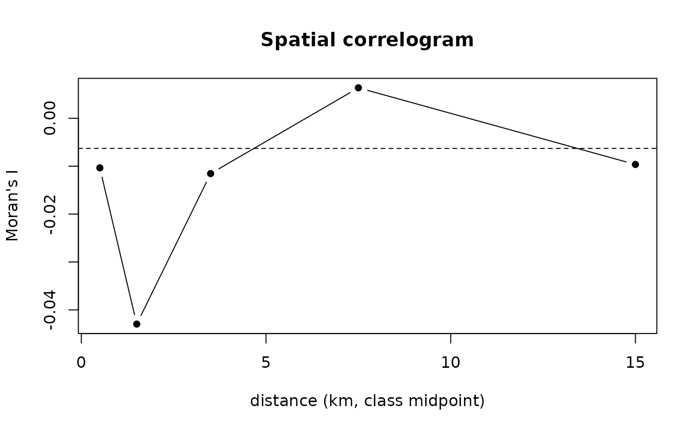
Moran's I by distance class: how far apart two points stop resembling each other.

For each class of distance, Moran's I of value over the pairs of points that far apart: the mean product of their deviations from the mean, over the variance. Near zero, points that far apart are as unlike as any two; the distance where it falls to zero is the scale blocks should exceed. For two models compared at the same points, value is the difference of their errors – the quantity whose mean is compared.

Usage

spatial_correlogram(
  x,
  y,
  value,
  breaks_km = c(0, 5, 10, 25, 50, 100, 200, 400, 800),
  coords = c("lonlat", "metres")
)

Arguments

x, y

Coordinates: longitude and latitude in degrees (great-circle distances) or metres (straight-line distances), as coords says.

value

One number per point.

breaks_km

The edges of the distance classes, in km.

coords

"lonlat" (the default) or "metres".

Value

A spatial_correlogram: a tibble with from_km, to_km, n_pairs, moran_i, and expected, Moran's I with no spatial structure (-1/(n-1)).

Examples

ex <- example_landscape()
obs <- ex$profiles$soc_stock
set.seed(1)
pred_a <- obs * exp(rnorm(length(obs), 0, 0.20))   # two models' predictions
pred_b <- obs * exp(rnorm(length(obs), 0, 0.25))
d <- abs(pred_a - obs) - abs(pred_b - obs)    # what a comparison of the two compares
cg <- spatial_correlogram(ex$profiles$x, ex$profiles$y, d,
                          breaks_km = c(0, 1, 2, 5, 10, 20))
cg
#> 
#> <spatial_correlogram> 160 point(s), Moran's I by distance class
#> # A tibble: 5 × 4
#>   from_km to_km n_pairs moran_i
#>     <dbl> <dbl>   <dbl>   <dbl>
#> 1       0     1     624  -0.01 
#> 2       1     2     521  -0.043
#> 3       2     5    1614  -0.012
#> 4       5    10    4328   0.006
#> 5      10    20    5563  -0.01 
#>   With no spatial structure, about -0.0063. Where it falls to that, points so far
#>   apart are as unlike as any two: the scale blocks should exceed.
plot(cg)